Today I am happy to announce that version 3.0.0 of my R mapping package choroplethr is now available from CRAN. To get it, you can simply type:
install.packages("choroplethr")
from an R console. If you don’t know what any of this means then I recommend taking Coursera’s excellent R Programming class 🙂
The most notable change in version 3.0.0 is that all functionality for handling zip codes has been deprecated and moved to a new package, choroplethrZip. I will have a separate post about that package later; here I just want to highlight changes to the main choroplethr package.
This change required me to break backwards compatability with previous versions of the package. This does not happen very often, so I took the opportunity to make other significant changes which had been building up.
A common request has always been to zoom further in. To support this for the county_choropleth function I broke the zoom parameter into two separate parameters: state_zoom and county_zoom. As an example, let’s make two choropleth maps:
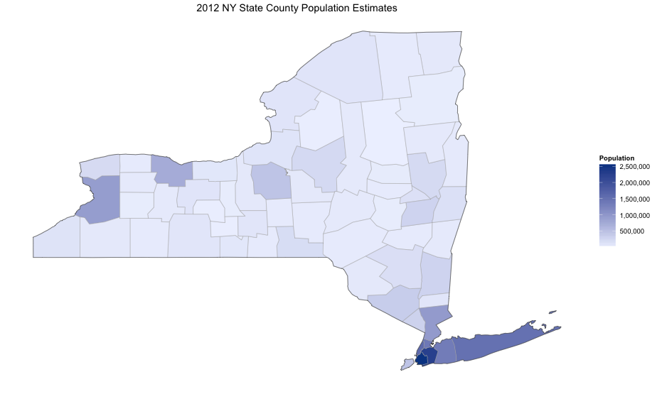
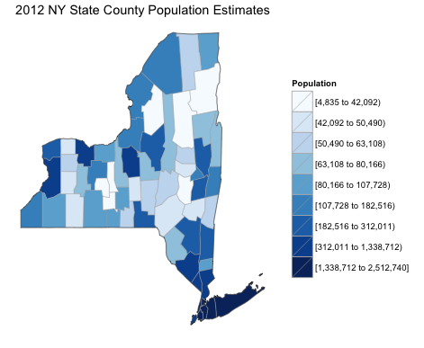
- The population of all counties in New York State
- The population of all counties in New York City
library(choroplethr)
data(df_pop_county)

county_choropleth(df_pop_county,
 title      = "2012 NY State County Population Estimates",
 legend     ="Population",
 num_colors = 1,
 state_zoom = "new york")
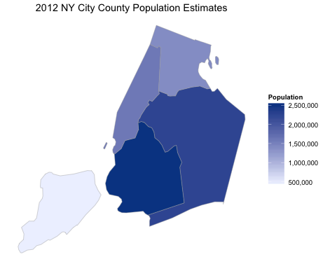
The image is informative: while there are a few high population counties in northern New York, the real population centers are the southern counties around New York City. However, they are so small that it is hard to tell which of the five counties in New York City is the most populous. We can zoom in on those counties by setting county_zoom to a vector of numeric FIPS County Codes.
# the county FIPS codes of the five counties that make up New York City
nyc_county_fips = c(36005, 36047, 36061, 36081, 36085)
county_choropleth(df_pop_county,
 title       = "2012 NY City County Population Estimates",
 legend      = "Population",
 num_colors  = 1,
 county_zoom = nyc_county_fips)
And now it is clear that Brooklyn and Queens are the most populated counties in New York City.
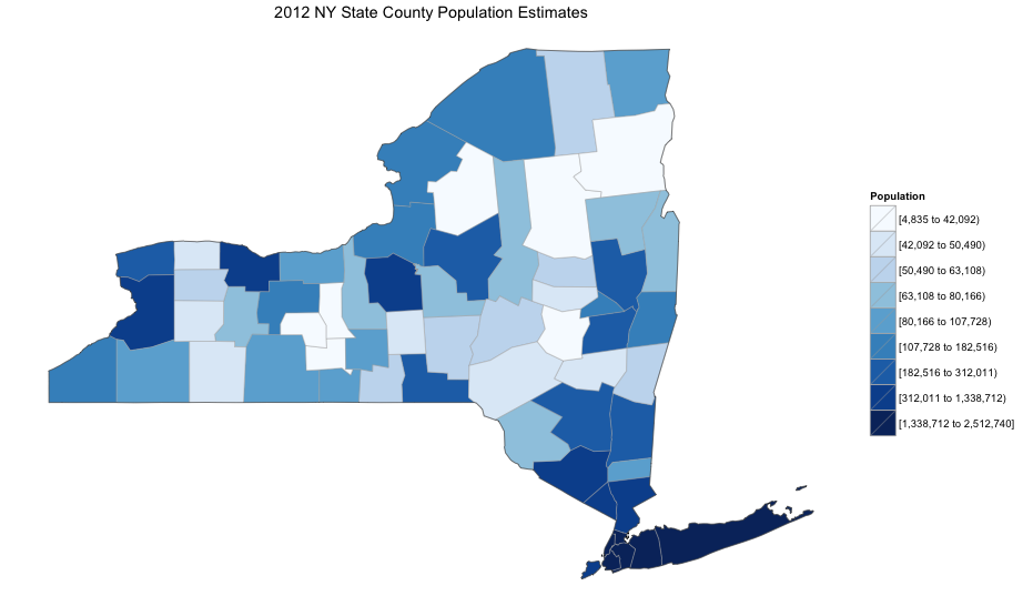
Users of past versions of choroplethr will note another change. The parameter that used to be called buckets is now called num_colors. I hope that this change will make it easier for users to understand exactly what the parameter does. By setting it to 1 we see a continuous scale. By setting it to any value in [2, 9] we see that many colors:
county_choropleth(df_pop_county,
 title      = "2012 NY State County Population Estimates",
 legend     = "Population",
 num_colors = 9,
 state_zoom = "new york")
The default value is still 7.
The choroplethr package used to support visualizing data from the US Census Bureau’s American Community Survey with the function choroplethr_acs. This function has now been broken up into two functions: state_choropleth_acs and county_choropleth_acs. Here are some examples of creating maps of US Per-capita Income. To learn more about the code B19301 (and how to find the codes of other interesting tables), see the article Mapping US Census Data.
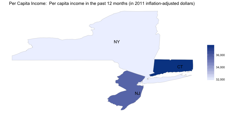
# Per capita income of New York, New Jersey and Connecticut.
states = c("new york", "new jersey", "connecticut")
state_choropleth_acs("B19301",
                     num_colors = 1,
                     zoom       = states)
To see more detail, we can look at the distribution of income in those states by county:
county_choropleth_acs("B19301",
                      num_colors = 1,
                      state_zoom = states)
As before, it is difficult to see the differences between the five counties that make up New York City. We can zoom in on those by setting the county_zoom parameter:
# see above for the definition of nyc_county_fips
county_choropleth_acs("B19301",
                      num_colors  = 1,
                      county_zoom = nyc_county_fips)
As always, if you create any interesting maps using choroplethr please consider sharing them with me either via twitter or the choroplethr google group.

