Today’s guest post is by R. Duncan McIntosh. Last week Duncan tweeted about using choroplethr to map the 2016 Florida primary election results. I’ve been wanting to analyze election results in R for some time, and asked Duncan to share with my readers how he did his analysis. This is his reply.
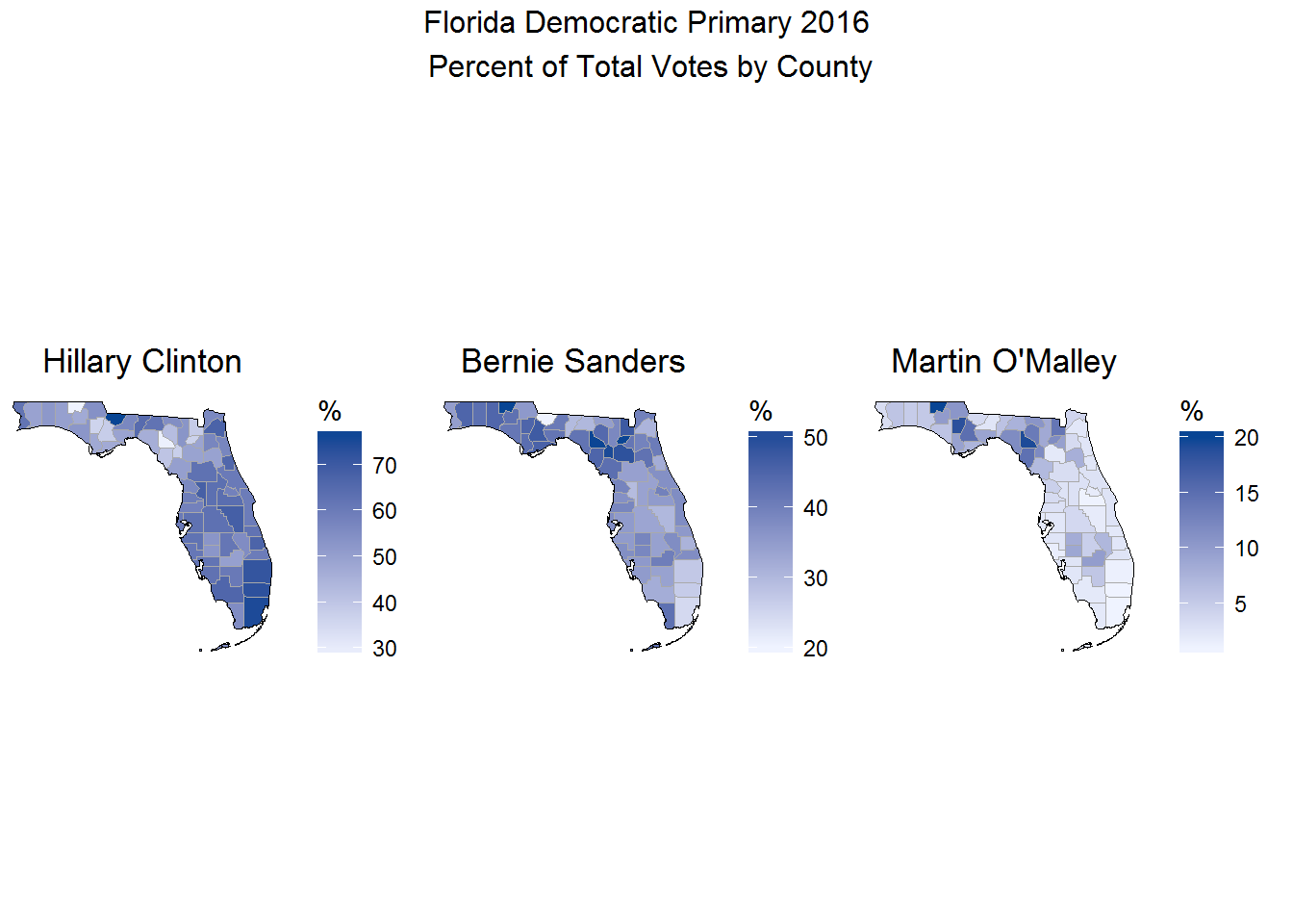
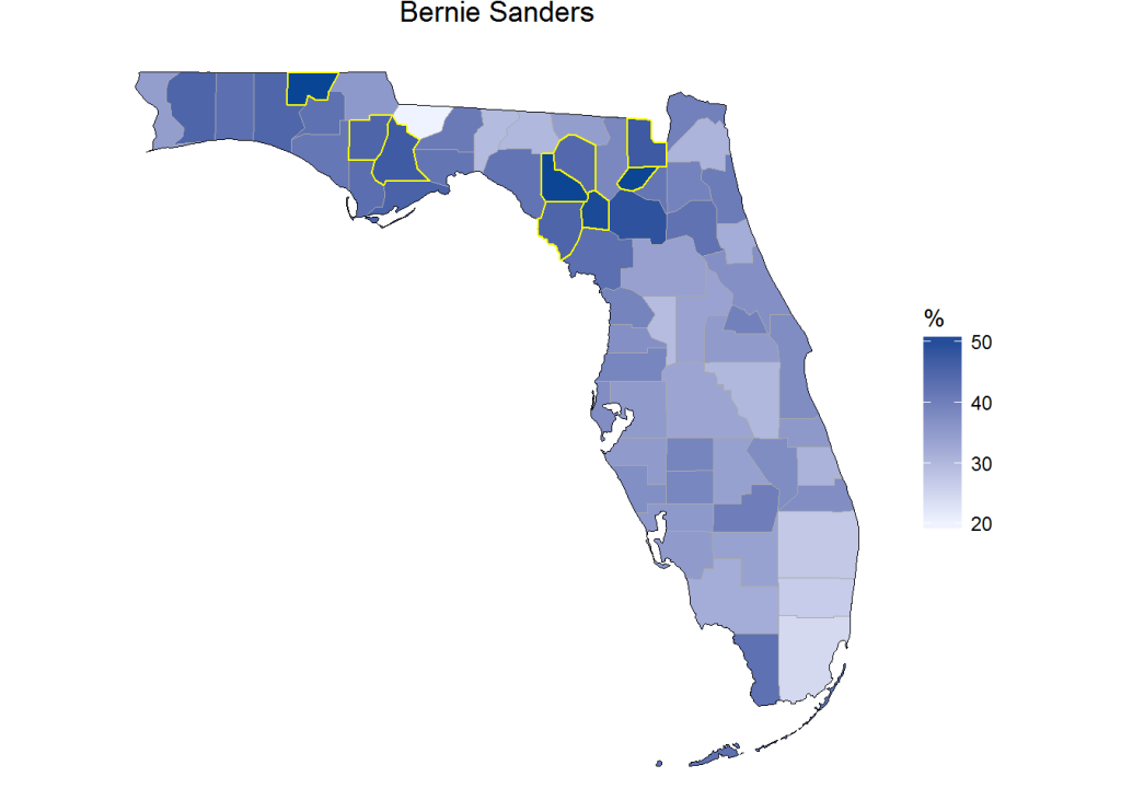
Election season is providing plenty of data to explore. Today I will demonstrate how to make a choropleth map of recent presidential primary election results in R. The final map we will produce compares the democratic candidates’ percent of total votes by county:

The Data
The election results for Florida are made available by Florida Election Watch. Using read.delim(), you can read directly from the tab delimited file online, which allows for a completely reproducible analysis from start to finish, though you might want to also download the file for offline use. Setting the argument strip.white = TRUE removes the problematic white spaces in the CountyNames column.
# Load required packages
library(ggplot2)
library(dplyr)
library(reshape2)
library(choroplethr)
library(choroplethrMaps)
library(gridExtra)
library(knitr)
# Read election results file from the web, and strip the white spaces
fl <- read.delim("http://fldoselectionfiles.elections.myflorida.com/enightfilespublic/20160315_ElecResultsFL.txt", strip.white = T)
Using the dplyr package, I filtered the data frame leaving only one party and selected only the columns I’m interested in. Using the reshape2 package’s dcast function, I then cast the data frame from long to wide format (i.e., with each candidate’s vote counts in a separate column). I also changed the datatype of the CountyName column to facilitate joining it with the county.regions data frame in a later step.
# Filter leaving only one party, and select desired columns
dem <- filter(fl, PartyCode == "DEM") %>% select(CountyName, CanNameLast, CanVotes)
# Cast dem dataframe from long to wide using dcast
dem_cast <- dcast(dem, CountyName ~ CanNameLast, sum)  # Now we can see each candidate's votes per county
colnames(dem_cast)[3] <- "OMalley" # Remove apostrophe from O'Malley
# Change CountyName column from Factor to lowercase Character
dem_cast$CountyName <- tolower(as.character(dem_cast$CountyName))
Then, I created a new column for each county’s total vote count and columns for each candidate’s percentage of those totals.
# Create columns for total votes in each county
dem_cast <- mutate(dem_cast, total = Clinton + OMalley + Sanders)
# Create columns for percentage variables
dem_cast <- mutate(dem_cast, hc = (Clinton/total)*100, bs = (Sanders/total)*100, mo = (OMalley/total)*100)
dem_cast[,6:8] <- round(dem_cast[,6:8], digits = 1)  # Round new variables to 1 decimal place
In order to map these county-level data with the choroplethr package, our data frame needs a column containing each county’s FIPS code. We can get this vector from the county.regions data frame supplied with the choroplethrMaps package. I filtered the county.regions data frame leaving only Florida counties, then selected the region column and the county.name column while renaming the latter to CountyName to match the analogous column in the dem_cast data frame. After joining these FIPS codes to our election results dataframe with a left_join(), our data frame is now ready for mapping.
# Read county.regions dataframe supplied by choroplethrMaps package
data("county.regions")
# Filter leaving only florida counties, and select only the 2 needed columns
fl.regions <- filter(county.regions, state.name == "florida") %>% select(region, "CountyName" = county.name)
# Join regions column from fl.regions dataframe to election results dataframe
df <- left_join(dem_cast, fl.regions)
A table view of counties won by Sanders:
bs.counties <- filter(df, Sanders > Clinton & Sanders > OMalley)
kable(bs.counties, caption = "Counties won by Sanders")
Counties won by Sanders
| baker |
654 |
240 |
805 |
1699 |
38.5 |
47.4 |
14.1 |
12003 |
| calhoun |
437 |
225 |
545 |
1207 |
36.2 |
45.2 |
18.6 |
12013 |
| dixie |
409 |
150 |
459 |
1018 |
40.2 |
45.1 |
14.7 |
12029 |
| gilchrist |
428 |
134 |
578 |
1140 |
37.5 |
50.7 |
11.8 |
12041 |
| holmes |
339 |
239 |
619 |
1197 |
28.3 |
51.7 |
20.0 |
12059 |
| lafayette |
204 |
136 |
363 |
703 |
29.0 |
51.6 |
19.3 |
12067 |
| liberty |
316 |
124 |
392 |
832 |
38.0 |
47.1 |
14.9 |
12077 |
| suwannee |
1475 |
475 |
1551 |
3501 |
42.1 |
44.3 |
13.6 |
12121 |
| union |
336 |
107 |
472 |
915 |
36.7 |
51.6 |
11.7 |
12125 |
A table view of counties won by Clinton:
hc.counties <- filter(df, Clinton > Sanders & Clinton > OMalley)
kable(hc.counties, caption = "Counties won by Clinton")
Counties won by Clinton
| alachua |
17777 |
708 |
17730 |
36215 |
49.1 |
49.0 |
2.0 |
12001 |
| bay |
5218 |
571 |
4134 |
9923 |
52.6 |
41.7 |
5.8 |
12005 |
| bradford |
1056 |
206 |
908 |
2170 |
48.7 |
41.8 |
9.5 |
12007 |
| brevard |
31862 |
1392 |
20100 |
53354 |
59.7 |
37.7 |
2.6 |
12009 |
| broward |
134328 |
1901 |
49054 |
185283 |
72.5 |
26.5 |
1.0 |
12011 |
| charlotte |
8126 |
321 |
4636 |
13083 |
62.1 |
35.4 |
2.5 |
12015 |
| citrus |
6865 |
555 |
4786 |
12206 |
56.2 |
39.2 |
4.5 |
12017 |
| clay |
5346 |
323 |
3699 |
9368 |
57.1 |
39.5 |
3.4 |
12019 |
| collier |
12719 |
390 |
6134 |
19243 |
66.1 |
31.9 |
2.0 |
12021 |
| columbia |
2304 |
372 |
1676 |
4352 |
52.9 |
38.5 |
8.5 |
12023 |
| desoto |
988 |
165 |
728 |
1881 |
52.5 |
38.7 |
8.8 |
12027 |
| duval |
59511 |
1982 |
27232 |
88725 |
67.1 |
30.7 |
2.2 |
12031 |
| escambia |
16770 |
853 |
9326 |
26949 |
62.2 |
34.6 |
3.2 |
12033 |
| flagler |
6160 |
215 |
2980 |
9355 |
65.8 |
31.9 |
2.3 |
12035 |
| franklin |
666 |
104 |
647 |
1417 |
47.0 |
45.7 |
7.3 |
12037 |
| gadsden |
7449 |
354 |
1945 |
9748 |
76.4 |
20.0 |
3.6 |
12039 |
| glades |
387 |
76 |
313 |
776 |
49.9 |
40.3 |
9.8 |
12043 |
| gulf |
568 |
111 |
520 |
1199 |
47.4 |
43.4 |
9.3 |
12045 |
| hamilton |
758 |
148 |
479 |
1385 |
54.7 |
34.6 |
10.7 |
12047 |
| hardee |
530 |
82 |
393 |
1005 |
52.7 |
39.1 |
8.2 |
12049 |
| hendry |
1157 |
104 |
647 |
1908 |
60.6 |
33.9 |
5.5 |
12051 |
| hernando |
8946 |
510 |
5549 |
15005 |
59.6 |
37.0 |
3.4 |
12053 |
| highlands |
3715 |
276 |
2056 |
6047 |
61.4 |
34.0 |
4.6 |
12055 |
| hillsborough |
69060 |
2402 |
38590 |
110052 |
62.8 |
35.1 |
2.2 |
12057 |
| indian river |
6901 |
228 |
3928 |
11057 |
62.4 |
35.5 |
2.1 |
12061 |
| jackson |
2805 |
551 |
1842 |
5198 |
54.0 |
35.4 |
10.6 |
12063 |
| jefferson |
1671 |
152 |
762 |
2585 |
64.6 |
29.5 |
5.9 |
12065 |
| lake |
15932 |
696 |
8482 |
25110 |
63.4 |
33.8 |
2.8 |
12069 |
| lee |
27993 |
1029 |
15673 |
44695 |
62.6 |
35.1 |
2.3 |
12071 |
| leon |
27401 |
1150 |
19930 |
48481 |
56.5 |
41.1 |
2.4 |
12073 |
| levy |
1570 |
215 |
1356 |
3141 |
50.0 |
43.2 |
6.8 |
12075 |
| madison |
1548 |
188 |
743 |
2479 |
62.4 |
30.0 |
7.6 |
12079 |
| manatee |
18129 |
696 |
10181 |
29006 |
62.5 |
35.1 |
2.4 |
12081 |
| marion |
18224 |
934 |
9896 |
29054 |
62.7 |
34.1 |
3.2 |
12083 |
| martin |
6526 |
278 |
4105 |
10909 |
59.8 |
37.6 |
2.5 |
12085 |
| miami-dade |
129546 |
1756 |
42052 |
173354 |
74.7 |
24.3 |
1.0 |
12086 |
| monroe |
4846 |
172 |
3755 |
8773 |
55.2 |
42.8 |
2.0 |
12087 |
| nassau |
2912 |
205 |
2062 |
5179 |
56.2 |
39.8 |
4.0 |
12089 |
| okaloosa |
4563 |
428 |
3788 |
8779 |
52.0 |
43.1 |
4.9 |
12091 |
| okeechobee |
1152 |
149 |
787 |
2088 |
55.2 |
37.7 |
7.1 |
12093 |
| orange |
66677 |
1148 |
36664 |
104489 |
63.8 |
35.1 |
1.1 |
12095 |
| osceola |
16533 |
431 |
7285 |
24249 |
68.2 |
30.0 |
1.8 |
12097 |
| palm beach |
103792 |
1957 |
39533 |
145282 |
71.4 |
27.2 |
1.3 |
12099 |
| pasco |
21772 |
1052 |
14505 |
37329 |
58.3 |
38.9 |
2.8 |
12101 |
| pinellas |
63716 |
2160 |
39767 |
105643 |
60.3 |
37.6 |
2.0 |
12103 |
| polk |
29345 |
1715 |
15492 |
46552 |
63.0 |
33.3 |
3.7 |
12105 |
| putnam |
3183 |
511 |
2747 |
6441 |
49.4 |
42.6 |
7.9 |
12107 |
| santa rosa |
3941 |
460 |
3612 |
8013 |
49.2 |
45.1 |
5.7 |
12113 |
| sarasota |
25896 |
681 |
15793 |
42370 |
61.1 |
37.3 |
1.6 |
12115 |
| seminole |
22089 |
688 |
15112 |
37889 |
58.3 |
39.9 |
1.8 |
12117 |
| st. johns |
9737 |
405 |
6956 |
17098 |
56.9 |
40.7 |
2.4 |
12109 |
| st. lucie |
17559 |
595 |
8098 |
26252 |
66.9 |
30.8 |
2.3 |
12111 |
| sumter |
7023 |
272 |
3022 |
10317 |
68.1 |
29.3 |
2.6 |
12119 |
| taylor |
987 |
251 |
908 |
2146 |
46.0 |
42.3 |
11.7 |
12123 |
| volusia |
26310 |
1174 |
16182 |
43666 |
60.3 |
37.1 |
2.7 |
12127 |
| wakulla |
1659 |
309 |
1424 |
3392 |
48.9 |
42.0 |
9.1 |
12129 |
| walton |
1515 |
158 |
1365 |
3038 |
49.9 |
44.9 |
5.2 |
12131 |
| washington |
858 |
182 |
781 |
1821 |
47.1 |
42.9 |
10.0 |
12133 |
O’Malley did not win any counties.
Mapping with Choroplethr
To create choropleth maps, choroplethr requires:
A data.frame with a column named “region” and a column named “value”. Elements in the “region” column must exactly match how regions are named in the “region” column in ?country.map.
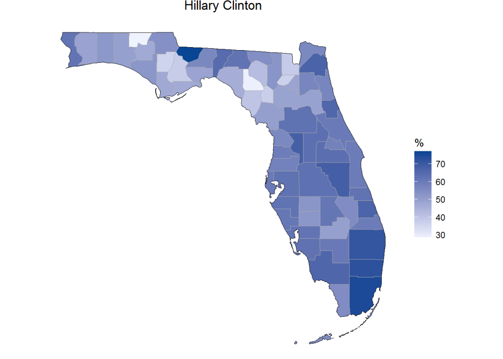
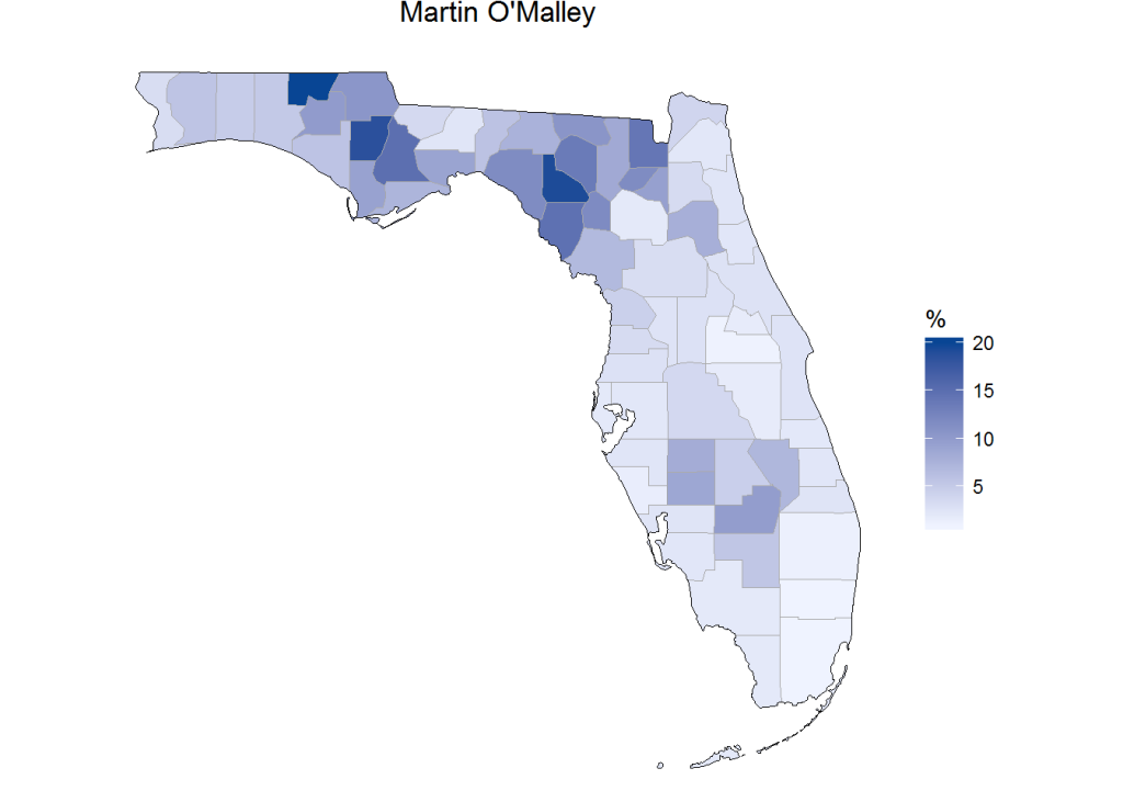
We have joined the regions directly from the county.map data frame, now we just need to add a column named value and assign it to equal the column we want to map. I do this with one line of base R immediately preceding each call of the county_choropleth() function. Below, I mapped each candidate’s percent of total vote by county in three separate maps, then all three in a row.
# For each candidate, map the percent of each counties' total vote using choroplethr package
df$value = df$bs  # Set the desired 'value' column for choroplethr
choro_bs = county_choropleth(df, state_zoom="florida", legend = "%", num_colors=1) +
  ggtitle("Bernie Sanders") +
  coord_map()  # Adds a Mercator projection
choro_bs

df$value = df$hc  # Set the desired 'value' column for choroplethr
choro_hc = county_choropleth(df, state_zoom="florida", legend = "%", num_colors=1) +
  ggtitle("Hillary Clinton") +
  coord_map()
choro_hc

df$value = df$mo  # Set the desired 'value' column for choroplethr
choro_mo = county_choropleth(df, state_zoom="florida", legend = "%", num_colors=1) +
  ggtitle("Martin O'Malley") +
  coord_map()
choro_mo

# Plot all three maps in a grid
grid.arrange(choro_hc, choro_bs, choro_mo, ncol=3, top = "Florida Democratic Primary 2016\n Percent of Total Votes by County\n ")

Highlight Counties
In this post, Ari shared a function for highlighting a county. Here, it’s applied to our first map:
# Function for highlighting a county
highlight_county = function(county_fips)
{
 library(choroplethrMaps)
 data(county.map, package="choroplethrMaps", envir=environment())
 df = county.map[county.map$region %in% county_fips, ]
 geom_polygon(data=df, aes(long, lat, group = group), color = "yellow", fill = NA, size = 0.5)
}
# Filter counties won by Sanders
bs.counties <- filter(df, Sanders > Clinton & Sanders > OMalley)
# Create list of counties won
bs.fips <- bs.counties[[9]]
# Map using the highlight_county() function after calling county_choropleth()
df$value = df$bs  # Set the desired 'value' column for choroplethr
choro_bs = county_choropleth(df, state_zoom="florida", legend = "%", num_colors=1) +
  highlight_county(bs.fips) +  # Highlight counties won
  ggtitle("Bernie Sanders") +
  coord_map()  # Adds a Mercator projection
choro_bs

Update
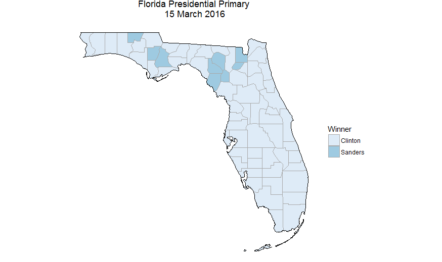
Ari asked if I’d add a map showing who won each county:
# Add a new column to show each county's winner
df$winner <- as.factor(ifelse(df$hc > df$bs, "Clinton", "Sanders"))
# Plot of winner by county</div>
df$value = df$winner  # Set the desired 'value' column for choroplethr
choro_winner = county_choropleth(df, state_zoom="florida", legend = "Winner", num_colors=2) +
  ggtitle("Florida Presidential Primary\n 15 March 2016") +
  coord_map()
choro_winner
