4 comments
Ari – thank you for the excellent package
Thank you for the kind words Michael!
Ari – very cool stuff.
Thank you!
Today I am happy to announce that a new version of choroplethr, v3.2.0, is now available. You can get it by typing the following from an R console:
install.packages("choroplethr")
Note that it sometimes takes a few days for new packages to get copied to each CRAN mirror. If install.packages(“choroplethr”) only gets you version 3.1.0, please try again tomorrow.
This version contains three changes.
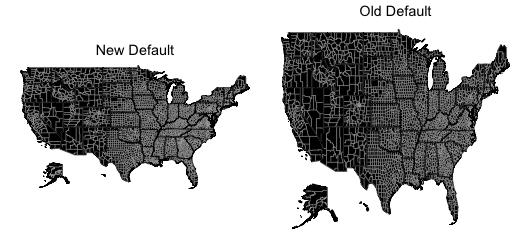
The most significant change is the addition of a better default map projection. I have discussed the issue of map projections in R at length here and here, among other places. Today I simply want to thank Hadley Wickham for pointing me to coord_quickmap(), which gives you a nice projection that also works with insets. Here is a comparison between the old and new maps:

library(choroplethr)

data(df_pop_county)
df_pop_county$value=NA

new = county_choropleth(df_pop_county,
                        title = "New Default")

old            = CountyChoropleth$new(df_pop_county)
old$title      = "Old Default"
old$projection = element_blank()
old            = old$render()

library(gridExtra)
grid.arrange(new, old, ncol=2)
On maps with many small regions, the borders can obscure information. Look at the map below, which shows all the zip codes in New York state.
In previous version of choroplethr it was hard to make the right-hand map. Choroplethr 3.2.0 simplifies this process quite a bit. It adds a ggplot_polygon member variable to the base Choropleth object. If you set it to geom_polygon(aes(fill=value), color=NA), as shown below, then the borders disappear:
library(choroplethrZip)
library(ggplot2)
data(df_pop_zip)

default = zip_choropleth(df_pop_zip,
                         state_zoom = "new york",
                         title = "With Border") +
            theme(legend.position="none")

c = ZipChoropleth$new(df_pop_zip)
c$title = "Without Border"
c$ggplot_polygon = geom_polygon(aes(fill = value),
                                color = NA)
c$set_zoom_zip(state_zoom  = "new york",
               county_zoom = NULL,
               msa_zoom    = NULL,
               zip_zoom    = NULL)

no_border = c$render() +
              theme(legend.position = "none")

grid.arrange(default, no_border, ncol = 2)
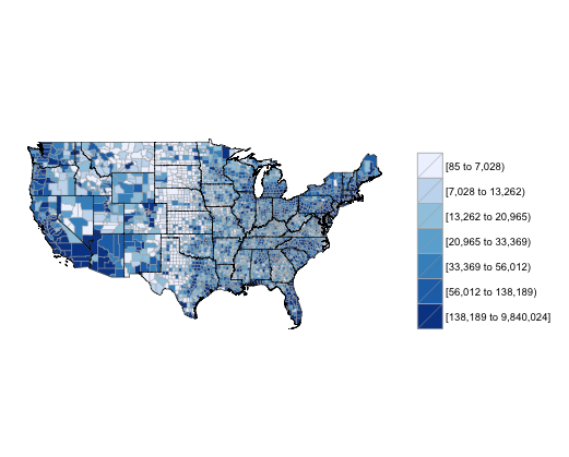
In my own work I frequently zoom in on the contiguous United States. I got tired of continually computing this vector of state names, so I added it as the variable continental_us_states. Here is an example:

data(df_pop_county)
data(continental_us_states)

county_choropleth(df_pop_county,
                  state_zoom = continental_us_states)
On Tuesday I wrote a guest blog post titled Following up on news stories with choroplethr and R on the Revolution Analytics blog. In it I describe how I used R and choroplethr to research how fracking has changed the demographics of North Dakota. I first learned about this issue in an interview that Russ Roberts did with Gregory Zuckerman on the EconTalk podcast. The post is of technical interest because I demonstrate how to calculate the percentage change in census demographics.
Ari – thank you for the excellent package
Thank you for the kind words Michael!
Ari – very cool stuff.
Thank you!